San Fransisco Bay Catch Dynamics

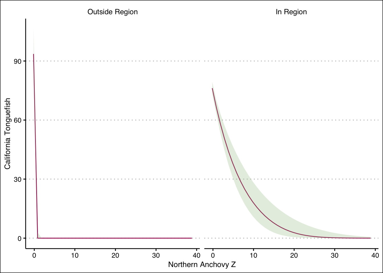
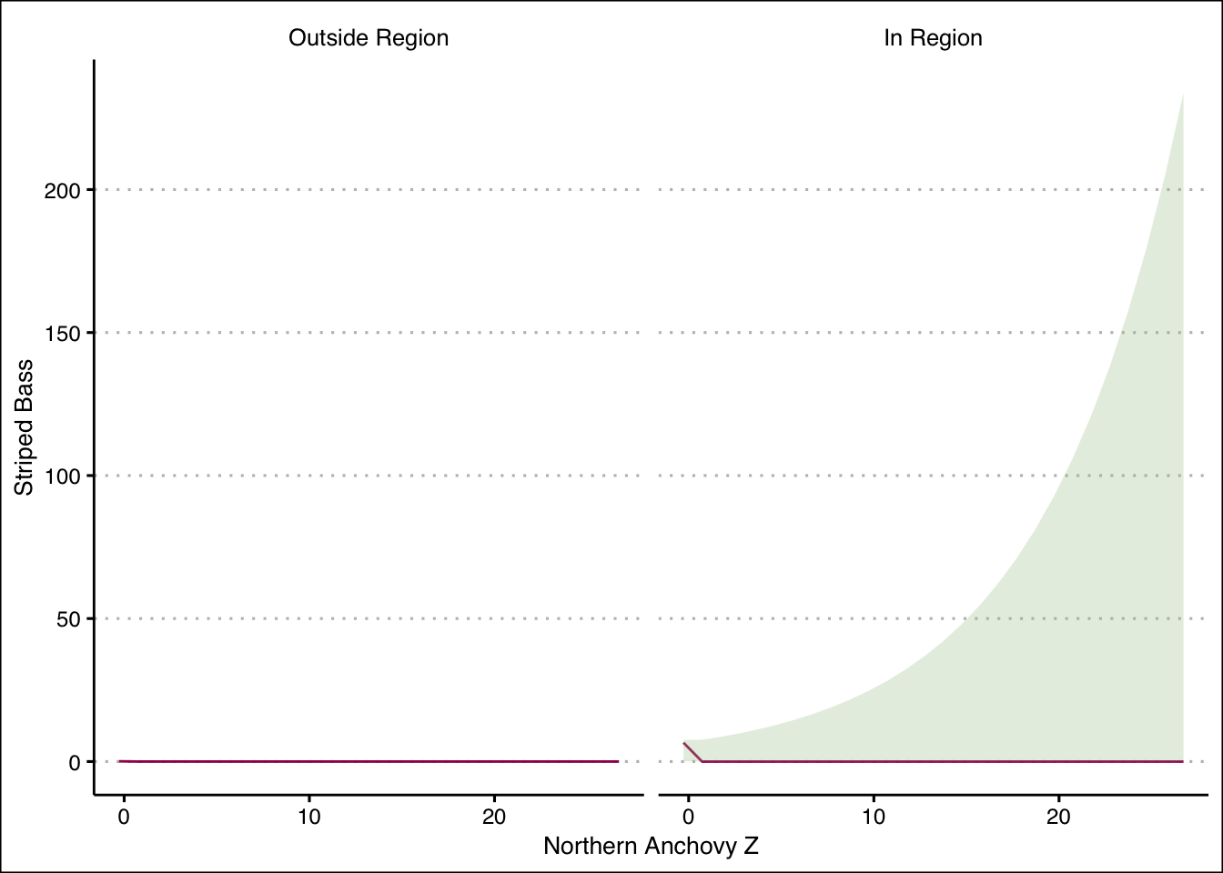
The San Francisco Bay is a large estuarine bay in Northern California which spans 60 miles (Britannica, n.d.). The San Francisco Estuary is the largest estuary in California, with rivers from the ridgeline of the Sierra Nevada mountains leading to the strait of the Golden Gate, including almost 60,000 square miles and nearly 40% of California (Partnership, n.d.). As of 2002, San Francisco Bay sustains nearly 500 species of fish, invertebrates, birds, mammals, insects and amphibians. It is an essential resting place, feeding area, and wintering ground for millions of birds on the Pacific Flyway. Nearly half of the state’s waterfowl and shorebirds and two-third of the state’s salmon pass through the Bay during their migrations (Conservation and Commission 2002).

In recent years harmful algal blooms (HABs) have decimated many populations in the bay. HABs are becoming more frequent and more intense across California as waters warm. Decreased flows from inland rivers and streams, and increased concentrations of nutrients and other land-based pollutants additionally exacerbate the growth of algae and cyanotoxins (Council 2022).

When monitoring the bay, it is often difficult to monitor less populated species to the extent of more frequent species. To combat this in this project I will be comparing populations of Northern Anchovy, the most populous species in the bay, to that of other more niche species. For example while we might catch thousands of Northern Anchovy in a season, there may be only one or two Tonguefish.

This project is organized in this way:

Directed Acyclic Graph
Data import and preliminary analysis
Indicator species analysis
Simulate data to test Hurdle model validity
Create function for Hurdle model
Call function on indicator species in the four regions of the bay:
- South Bay
- Central Bay
- San Pablo Bay
- Suisun Bay

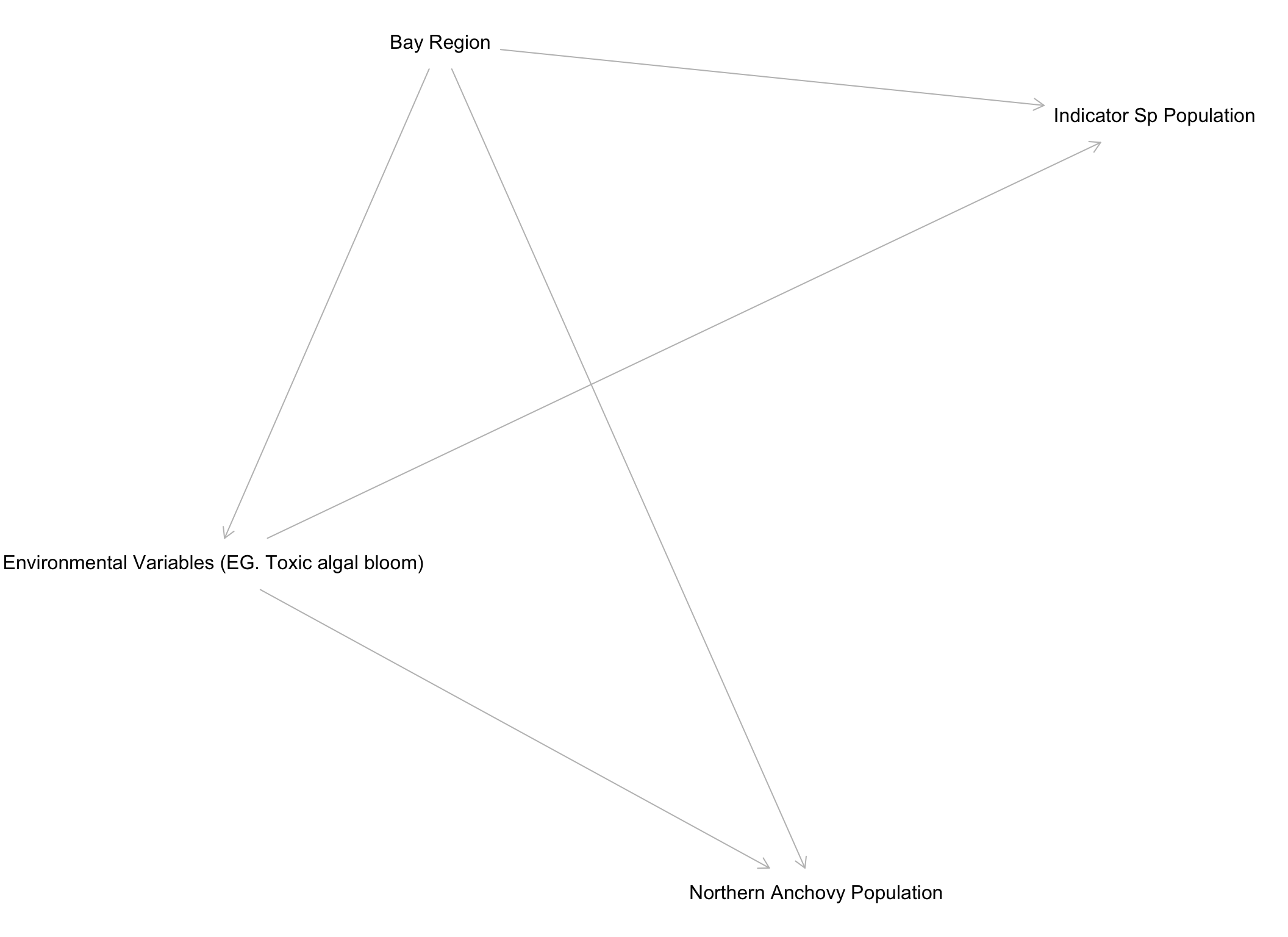
DAG

This analysis is predicated on the same environmental factors effecting Northern Anchovies and other species at similar levels. This leads to a DAG which looks like this:

Code

dag <- dagitty::dagitty('dag {
bb="0,0,1,1"
"Bay Region" [pos="0.375,0.496"]
"Environmental Variables (EG. Toxic algal bloom)" [pos="0.378,0.222"]
"Northern Anchovy Population" [pos="0.277,0.343"]
"Indicator Sp Population" [pos="0.495,0.341"]
"Bay Region" -> "Environmental Variables (EG. Toxic algal bloom)"
"Bay Region" -> "Northern Anchovy Population"
"Bay Region" -> "Indicator Sp Population"
"Environmental Variables (EG. Toxic algal bloom)" -> "Northern Anchovy Population"
"Environmental Variables (EG. Toxic algal bloom)" -> "Indicator Sp Population"
}')

par(mar = c(5,5,5,5))
plot(dagitty::graphLayout(dag))

Import packages

Code

pacman::p_load('tidyverse', 
               'here',
               'janitor',
               'indicspecies',
               'MASS',
               'ggthemes',
               'stargazer',
               'broom',
               'knitr',
               'kableExtra',
               'htmltools')

Import and clean data

First we import data which was requested from (Institute n.d.). This data encapsulates individual otter trawls which were taken in the Bay between 1972 and 2017. The net is kept in the water for 5 minutes and then retrieved. A majority of the trawls are taken in the South Bay, however there are consistent year over year trawls in the other regions (Central bay, San Pablo bay, and Suisun bay).

Code

# Raw catch data
catch_raw <- read_csv(here::here('posts', 'sf_bay_catches', 'data', 'catch_9218.csv'))

# For easy reference we also import species key 
species_key <- read_csv(here::here('posts', 'sf_bay_catches','data', 'species_key.csv'), col_names = FALSE)

Now we can clean up the messy dataset and make a functional species key

Code

# The species key has some very difficult first columns so we need to restrict it down to just species code and name
species_key_clean <- species_key[c(4,5),3:125] %>% 
  row_to_names(row_number = 1) %>% 
  clean_names() %>% 
  remove_empty(which = "rows") %>% 
  pivot_longer(cols = everything(),names_to = 'species_code', values_to = 'species_name')%>% 
  mutate(species_code = str_to_upper(species_code),
                                     species_name = str_to_title(str_to_lower(species_name)))

species_key_clean %>% 
   kable( format = "html", digits = 3,
      caption = "Species Key") %>% 
  kable_styling(
    bootstrap_options = c("striped", "hover", "condensed", "responsive"),
    full_width = FALSE,
    position   = "center",
    font_size  = 14
  ) %>% 
  row_spec(0, bold = TRUE, color = "white", background = "#A0185A") %>%  # header
  row_spec(1:nrow(species_key_clean), color = "black", background = "#FFC4EB") %>% 
  scroll_box(width = "300px", height = "600px")

Species Key
species_code	species_name
AG	Arrow Goby
AS	American Shad
BBC	Brown Bullhead Catfish
BG	Bay Goby
BHS	Bonyhead Sculpin
BOC	Bocaccio Rockfish
BP	Black Perch
BPF	Bay Pipefish
BR	Bat Ray
BRF	Bolinas Rockfish
BRO	Brown Rockfish
BS	Brown Smoothhound
BSC	Buffalo Sculpin
BSF	Blacktail Snailfish
BSK	Big Skate
BSP	Barred Surfperch
CAL	Calico Surfperch
CBZ	Cabezon
CG	Chameleon Goby
CH	California Halibut
CLF	California Lizardfish
COT	C-O Turbot
CRF	Copper Rockfish
CRL	Curlfin Turbot
CSG	Cheekspot Goby
CT	California Tonguefish
DS	Dover Sole
DSP	Dwarf Surfperch
DT	Diamond Turbot
EP	Eel Pout
ES	English Sole
GBY	Goby Sp.
GRF	Grass Rockfish
GRU	Calif (Silverside) Grunion
GS	Green Sturgeon
HB	Halibut Sp.
HH	Hornyhead Turbot
HMP	Half Moon Perch
JS	Jacksmelt
KF	Kelp Fish
KG	Kelp Greenling
KP	Kelp Pipefish
KS	King Salmon
LC	Ling Cod
LFS	Longfin Smelt
LS	Leopard Shark
LSD	Longfin Sanddab
MFE	Monkey Face Eel
MS	Mudsucker
NA	Northern Anchovy
NEW	NA
NMS	Northern Midshipman
NS	Night Smelt
PB	Pacific Butterfish
PEN	Penpoint Gunnel
PER	Pacific Electric Ray
PH	Pacific Herring
PHB	Pacific Halibut
PL	Pacific Lamprey
PM	Pacific Mackerel
PMS	Plainfin Midshipman
POM	Pompano
PP	Prickleback
PS	Pacific Sardine
PSD	Pacific Sanddab
PSP	Pile Surfperch
PT	Pacific Tomcod
RED	Redtail Surfperch
RF	Rockfish
RH	Round Herring
RL	Red Irish Lord
RP	Reef Perch
RS	Rex Sole
RSP	Rainbow Surfperch
RUB	Rubberlip Surfperch
SAL	Salmon Species
SB	Striped Bass
SBG	Saddleback Gunnel
SC	Sculpin Sp.
SCA	Scalyfin Sole
SD	Sanddab Sp.
SDF	Spiny Dogfish
SF	Starry Flounder
SFS	Spotfin Surfperch
SGF	Shovelnose Guitarfish
SGS	Sevengill Shark
SH	Unidentified Shad
SHI	Shimofuri Goby
SHO	Shokihaze Gobi
SHS	Staghorn Sculpin
SIL	Silver Surfperch
SIS	Silverside
SKF	Spotted Kelpfish
SM	Smelt Sp.
SMS	Specked Fin Midshipman
SN	Snailfish Sp.
SPT	Spotted Turbot
SS	Sand Sole
SSD	Speckled Sanddab
SSN	Showy Snailfish
SSP	Shiner Surfperch
STU	Sturgeon Species
SUR	Surf Smelt
TC	Tomcod
TFS	Threadfin Shad
THS	Thorny Sculpin
TP	Tule Perch
TPS	Tidepool Sculpin
TR	Thornback Ray
TS	Topsmelt
TSS	Three Spine Stickleback
UG	Unknown Goby Species
UMS	Unidentified Midshipman
US	Unknown Sole Species
USP	Surfperch, Species Unknown
WBS	Whitebait Smelt
WC	White Croaker
WHS	White Surfperch
WS	White Sturgeon
WSB	White Seabass
WSP	Walleye Surfperch
YG	Yellowfin Goby
YR	Yellowtail Rockfish

Code

# The catch data is much cleaner, all we need is a quick clean names
catch_clean <- catch_raw %>% 
  clean_names()

catch_clean$species_code[is.na(catch_clean$species_code)] <- 'NA'

catch_clean %>% 
  head(100) %>% 
  kable( format = "html", digits = 3,
      caption = tags$caption(
      "100 Rows of Catch Data",
      style = "caption-side: top; text-align: left; font-weight: bold; color: #A0185A; font-size: 16px;"
    )) %>% 
  kable_styling(
    bootstrap_options = c("striped", "hover", "condensed", "responsive"),
    full_width = FALSE,
    position   = "left",
    font_size  = 14
  ) %>% 
  row_spec(0, bold = TRUE, color = "white", background = "#A0185A") %>%  # header
  scroll_box(width = "800px", height = "300px")


catch_info_trawl_id	species_code	size	class	number	sex	trawl_map_trawl_id	locale	trawl_map_training_trawl	trawl_map_data_audit	expr1	expr2	trawl_info_trawl_id	hydro_id	scientists	intern	date	school	trawl_time_begin	trawl_time_end	trawl_time_total	depth_of_trawl	tidal_current	last_slack_time	last_slack_tide	last_slack_height	sample_station	water_type	substrate	net_drag_bottom	line_length	start_latitude	start_longitude	end_latitude	end_longitude	field0	field1
10	SSP	0	NA	1	NA	10	SOUTH BAY	NA	NA	1992	10	10	NA	KRISTEN	ANTOINETTE	01-Oct-92	WALT DISNEY	1340	1355	15	6.40	EBB	NA	NA	NA	NA	SHOAL	SHELLS	TRUE	30	NA	NA	NA	NA	NA	NA
10	SSP	90	NA	1	NA	10	SOUTH BAY	NA	NA	1992	10	10	NA	KRISTEN	ANTOINETTE	01-Oct-92	WALT DISNEY	1340	1355	15	6.40	EBB	NA	NA	NA	NA	SHOAL	SHELLS	TRUE	30	NA	NA	NA	NA	NA	NA
10	SSP	56	NA	1	NA	10	SOUTH BAY	NA	NA	1992	10	10	NA	KRISTEN	ANTOINETTE	01-Oct-92	WALT DISNEY	1340	1355	15	6.40	EBB	NA	NA	NA	NA	SHOAL	SHELLS	TRUE	30	NA	NA	NA	NA	NA	NA
10	NA	NA	NA	15	NA	10	SOUTH BAY	NA	NA	1992	10	10	NA	KRISTEN	ANTOINETTE	01-Oct-92	WALT DISNEY	1340	1355	15	6.40	EBB	NA	NA	NA	NA	SHOAL	SHELLS	TRUE	30	NA	NA	NA	NA	NA	NA
10	CH	NA	NA	4	NA	10	SOUTH BAY	NA	NA	1992	10	10	NA	KRISTEN	ANTOINETTE	01-Oct-92	WALT DISNEY	1340	1355	15	6.40	EBB	NA	NA	NA	NA	SHOAL	SHELLS	TRUE	30	NA	NA	NA	NA	NA	NA
10	BS	480	NA	1	F	10	SOUTH BAY	NA	NA	1992	10	10	NA	KRISTEN	ANTOINETTE	01-Oct-92	WALT DISNEY	1340	1355	15	6.40	EBB	NA	NA	NA	NA	SHOAL	SHELLS	TRUE	30	NA	NA	NA	NA	NA	NA
10	BS	370	NA	1	M	10	SOUTH BAY	NA	NA	1992	10	10	NA	KRISTEN	ANTOINETTE	01-Oct-92	WALT DISNEY	1340	1355	15	6.40	EBB	NA	NA	NA	NA	SHOAL	SHELLS	TRUE	30	NA	NA	NA	NA	NA	NA
10	PMS	NA	NA	4	NA	10	SOUTH BAY	NA	NA	1992	10	10	NA	KRISTEN	ANTOINETTE	01-Oct-92	WALT DISNEY	1340	1355	15	6.40	EBB	NA	NA	NA	NA	SHOAL	SHELLS	TRUE	30	NA	NA	NA	NA	NA	NA
10	SSP	NA	NA	2	NA	10	SOUTH BAY	NA	NA	1992	10	10	NA	KRISTEN	ANTOINETTE	01-Oct-92	WALT DISNEY	1340	1355	15	6.40	EBB	NA	NA	NA	NA	SHOAL	SHELLS	TRUE	30	NA	NA	NA	NA	NA	NA
10	LS	460	46	1	M	10	SOUTH BAY	NA	NA	1992	10	10	NA	KRISTEN	ANTOINETTE	01-Oct-92	WALT DISNEY	1340	1355	15	6.40	EBB	NA	NA	NA	NA	SHOAL	SHELLS	TRUE	30	NA	NA	NA	NA	NA	NA
10	BR	615	62	1	M	10	SOUTH BAY	NA	NA	1992	10	10	NA	KRISTEN	ANTOINETTE	01-Oct-92	WALT DISNEY	1340	1355	15	6.40	EBB	NA	NA	NA	NA	SHOAL	SHELLS	TRUE	30	NA	NA	NA	NA	NA	NA
11	NA	NA	NA	20	NA	11	SOUTH BAY	NA	NA	1992	10	11	NA	TANYA	ANTOINETTE	01-Oct-92	WALT DISNEY	1540	1555	15	6.40	NA	NA	NA	NA	NA	NA	NA	TRUE	NA	NA	NA	NA	NA	NA	NA
11	PMS	NA	NA	8	NA	11	SOUTH BAY	NA	NA	1992	10	11	NA	TANYA	ANTOINETTE	01-Oct-92	WALT DISNEY	1540	1555	15	6.40	NA	NA	NA	NA	NA	NA	NA	TRUE	NA	NA	NA	NA	NA	NA	NA
14	NA	NA	NA	2	NA	14	SOUTH BAY	NA	NA	1992	10	14	NA	RENAE	LISA MARIE	02-Oct-92	WALT DISNEY	1350	1405	15	3.00	FLOOD	1232	NA	NA	E	SHOAL	NA	TRUE	NA	NA	NA	NA	NA	NA	NA
14	CH	NA	NA	15	NA	14	SOUTH BAY	NA	NA	1992	10	14	NA	RENAE	LISA MARIE	02-Oct-92	WALT DISNEY	1350	1405	15	3.00	FLOOD	1232	NA	NA	E	SHOAL	NA	TRUE	NA	NA	NA	NA	NA	NA	NA
14	PMS	NA	NA	7	NA	14	SOUTH BAY	NA	NA	1992	10	14	NA	RENAE	LISA MARIE	02-Oct-92	WALT DISNEY	1350	1405	15	3.00	FLOOD	1232	NA	NA	E	SHOAL	NA	TRUE	NA	NA	NA	NA	NA	NA	NA
14	SSP	NA	NA	6	NA	14	SOUTH BAY	NA	NA	1992	10	14	NA	RENAE	LISA MARIE	02-Oct-92	WALT DISNEY	1350	1405	15	3.00	FLOOD	1232	NA	NA	E	SHOAL	NA	TRUE	NA	NA	NA	NA	NA	NA	NA
17	YG	NA	NA	2	NA	17	SOUTH BAY	NA	NA	1992	10	17	NA	EGP	LISA MARIE	02-Oct-92	WALT DISNEY	1445	1500	15	5.00	FLOOD	1232	NA	NA	I	SHOAL	NA	TRUE	30	NA	NA	NA	NA	NA	NA
17	BR	430	44	1	F	17	SOUTH BAY	NA	NA	1992	10	17	NA	EGP	LISA MARIE	02-Oct-92	WALT DISNEY	1445	1500	15	5.00	FLOOD	1232	NA	NA	I	SHOAL	NA	TRUE	30	NA	NA	NA	NA	NA	NA
17	CG	NA	NA	3	NA	17	SOUTH BAY	NA	NA	1992	10	17	NA	EGP	LISA MARIE	02-Oct-92	WALT DISNEY	1445	1500	15	5.00	FLOOD	1232	NA	NA	I	SHOAL	NA	TRUE	30	NA	NA	NA	NA	NA	NA
17	NA	NA	NA	31	NA	17	SOUTH BAY	NA	NA	1992	10	17	NA	EGP	LISA MARIE	02-Oct-92	WALT DISNEY	1445	1500	15	5.00	FLOOD	1232	NA	NA	I	SHOAL	NA	TRUE	30	NA	NA	NA	NA	NA	NA
17	CH	NA	NA	7	NA	17	SOUTH BAY	NA	NA	1992	10	17	NA	EGP	LISA MARIE	02-Oct-92	WALT DISNEY	1445	1500	15	5.00	FLOOD	1232	NA	NA	I	SHOAL	NA	TRUE	30	NA	NA	NA	NA	NA	NA
18	SSD	NA	NA	5	NA	18	SOUTH BAY	NA	NA	1992	10	18	NA	CAROL	LISA MARIE	02-Oct-92	WALT DISNEY	1540	1555	15	10.00	FLOOD	NA	NA	NA	J-5	CHANNEL	MUD	TRUE	30	NA	NA	NA	NA	NA	NA
18	CH	NA	NA	4	NA	18	SOUTH BAY	NA	NA	1992	10	18	NA	CAROL	LISA MARIE	02-Oct-92	WALT DISNEY	1540	1555	15	10.00	FLOOD	NA	NA	NA	J-5	CHANNEL	MUD	TRUE	30	NA	NA	NA	NA	NA	NA
18	YG	NA	NA	4	NA	18	SOUTH BAY	NA	NA	1992	10	18	NA	CAROL	LISA MARIE	02-Oct-92	WALT DISNEY	1540	1555	15	10.00	FLOOD	NA	NA	NA	J-5	CHANNEL	MUD	TRUE	30	NA	NA	NA	NA	NA	NA
18	NA	NA	NA	5	NA	18	SOUTH BAY	NA	NA	1992	10	18	NA	CAROL	LISA MARIE	02-Oct-92	WALT DISNEY	1540	1555	15	10.00	FLOOD	NA	NA	NA	J-5	CHANNEL	MUD	TRUE	30	NA	NA	NA	NA	NA	NA
18	PMS	NA	NA	40	NA	18	SOUTH BAY	NA	NA	1992	10	18	NA	CAROL	LISA MARIE	02-Oct-92	WALT DISNEY	1540	1555	15	10.00	FLOOD	NA	NA	NA	J-5	CHANNEL	MUD	TRUE	30	NA	NA	NA	NA	NA	NA
18	CG	NA	NA	4	NA	18	SOUTH BAY	NA	NA	1992	10	18	NA	CAROL	LISA MARIE	02-Oct-92	WALT DISNEY	1540	1555	15	10.00	FLOOD	NA	NA	NA	J-5	CHANNEL	MUD	TRUE	30	NA	NA	NA	NA	NA	NA
19	SSP	NA	NA	14	NA	19	SOUTH BAY	NA	NA	1992	10	19	2	CAROL	DAVE	03-Oct-92	TEACHER SEMINAR	859	915	16	5.67	EBB	822	NA	NA	C-2	SHOAL	NA	TRUE	30	NA	NA	NA	NA	NA	NA
19	SS	NA	NA	2	NA	19	SOUTH BAY	NA	NA	1992	10	19	2	CAROL	DAVE	03-Oct-92	TEACHER SEMINAR	859	915	16	5.67	EBB	822	NA	NA	C-2	SHOAL	NA	TRUE	30	NA	NA	NA	NA	NA	NA
19	DT	NA	NA	3	NA	19	SOUTH BAY	NA	NA	1992	10	19	2	CAROL	DAVE	03-Oct-92	TEACHER SEMINAR	859	915	16	5.67	EBB	822	NA	NA	C-2	SHOAL	NA	TRUE	30	NA	NA	NA	NA	NA	NA
19	CH	NA	NA	35	NA	19	SOUTH BAY	NA	NA	1992	10	19	2	CAROL	DAVE	03-Oct-92	TEACHER SEMINAR	859	915	16	5.67	EBB	822	NA	NA	C-2	SHOAL	NA	TRUE	30	NA	NA	NA	NA	NA	NA
19	PMS	NA	NA	60	NA	19	SOUTH BAY	NA	NA	1992	10	19	2	CAROL	DAVE	03-Oct-92	TEACHER SEMINAR	859	915	16	5.67	EBB	822	NA	NA	C-2	SHOAL	NA	TRUE	30	NA	NA	NA	NA	NA	NA
19	NA	NA	NA	101	NA	19	SOUTH BAY	NA	NA	1992	10	19	2	CAROL	DAVE	03-Oct-92	TEACHER SEMINAR	859	915	16	5.67	EBB	822	NA	NA	C-2	SHOAL	NA	TRUE	30	NA	NA	NA	NA	NA	NA
20	NA	NA	NA	750	NA	20	SOUTH BAY	NA	NA	1992	10	20	3	SUSAN	DAVE	03-Oct-92	TEACHER SEMINAR	945	1000	15	5.00	EBB	822	NA	NA	E	SHOAL	SHELLS	TRUE	30	NA	NA	NA	NA	NA	NA
20	CH	NA	NA	4	NA	20	SOUTH BAY	NA	NA	1992	10	20	3	SUSAN	DAVE	03-Oct-92	TEACHER SEMINAR	945	1000	15	5.00	EBB	822	NA	NA	E	SHOAL	SHELLS	TRUE	30	NA	NA	NA	NA	NA	NA
20	PMS	NA	NA	6	NA	20	SOUTH BAY	NA	NA	1992	10	20	3	SUSAN	DAVE	03-Oct-92	TEACHER SEMINAR	945	1000	15	5.00	EBB	822	NA	NA	E	SHOAL	SHELLS	TRUE	30	NA	NA	NA	NA	NA	NA
20	BG	NA	NA	3	NA	20	SOUTH BAY	NA	NA	1992	10	20	3	SUSAN	DAVE	03-Oct-92	TEACHER SEMINAR	945	1000	15	5.00	EBB	822	NA	NA	E	SHOAL	SHELLS	TRUE	30	NA	NA	NA	NA	NA	NA
20	BSP	NA	NA	3	NA	20	SOUTH BAY	NA	NA	1992	10	20	3	SUSAN	DAVE	03-Oct-92	TEACHER SEMINAR	945	1000	15	5.00	EBB	822	NA	NA	E	SHOAL	SHELLS	TRUE	30	NA	NA	NA	NA	NA	NA
20	SHS	NA	NA	2	NA	20	SOUTH BAY	NA	NA	1992	10	20	3	SUSAN	DAVE	03-Oct-92	TEACHER SEMINAR	945	1000	15	5.00	EBB	822	NA	NA	E	SHOAL	SHELLS	TRUE	30	NA	NA	NA	NA	NA	NA
20	SSP	NA	NA	10	NA	20	SOUTH BAY	NA	NA	1992	10	20	3	SUSAN	DAVE	03-Oct-92	TEACHER SEMINAR	945	1000	15	5.00	EBB	822	NA	NA	E	SHOAL	SHELLS	TRUE	30	NA	NA	NA	NA	NA	NA
21	NA	NA	NA	18	NA	21	SOUTH BAY	NA	NA	1992	10	21	4	LISA	DAVE	03-Oct-92	TEACHER SEMINAR	1035	1050	15	7.60	EBB	822	NA	NA	F	SHOAL	SHELLS	TRUE	30	NA	NA	NA	NA	NA	NA
21	SSP	NA	NA	10	NA	21	SOUTH BAY	NA	NA	1992	10	21	4	LISA	DAVE	03-Oct-92	TEACHER SEMINAR	1035	1050	15	7.60	EBB	822	NA	NA	F	SHOAL	SHELLS	TRUE	30	NA	NA	NA	NA	NA	NA
21	CG	NA	NA	18	NA	21	SOUTH BAY	NA	NA	1992	10	21	4	LISA	DAVE	03-Oct-92	TEACHER SEMINAR	1035	1050	15	7.60	EBB	822	NA	NA	F	SHOAL	SHELLS	TRUE	30	NA	NA	NA	NA	NA	NA
21	CH	NA	NA	8	NA	21	SOUTH BAY	NA	NA	1992	10	21	4	LISA	DAVE	03-Oct-92	TEACHER SEMINAR	1035	1050	15	7.60	EBB	822	NA	NA	F	SHOAL	SHELLS	TRUE	30	NA	NA	NA	NA	NA	NA
21	SHS	NA	NA	7	NA	21	SOUTH BAY	NA	NA	1992	10	21	4	LISA	DAVE	03-Oct-92	TEACHER SEMINAR	1035	1050	15	7.60	EBB	822	NA	NA	F	SHOAL	SHELLS	TRUE	30	NA	NA	NA	NA	NA	NA
21	PMS	NA	NA	3	NA	21	SOUTH BAY	NA	NA	1992	10	21	4	LISA	DAVE	03-Oct-92	TEACHER SEMINAR	1035	1050	15	7.60	EBB	822	NA	NA	F	SHOAL	SHELLS	TRUE	30	NA	NA	NA	NA	NA	NA
23	NA	NA	7	2	NA	23	SOUTH BAY	NA	NA	1992	10	23	NA	EGP	DAVE	05-Oct-92	BOLLINGER	840	857	17	NA	NA	NA	NA	NA	D-3	SHOAL	SHELLS	TRUE	66	NA	NA	NA	NA	NA	NA
23	SSP	NA	8	1	NA	23	SOUTH BAY	NA	NA	1992	10	23	NA	EGP	DAVE	05-Oct-92	BOLLINGER	840	857	17	NA	NA	NA	NA	NA	D-3	SHOAL	SHELLS	TRUE	66	NA	NA	NA	NA	NA	NA
23	CG	NA	7	2	NA	23	SOUTH BAY	NA	NA	1992	10	23	NA	EGP	DAVE	05-Oct-92	BOLLINGER	840	857	17	NA	NA	NA	NA	NA	D-3	SHOAL	SHELLS	TRUE	66	NA	NA	NA	NA	NA	NA
23	CG	NA	6	4	NA	23	SOUTH BAY	NA	NA	1992	10	23	NA	EGP	DAVE	05-Oct-92	BOLLINGER	840	857	17	NA	NA	NA	NA	NA	D-3	SHOAL	SHELLS	TRUE	66	NA	NA	NA	NA	NA	NA
23	CG	NA	5	10	NA	23	SOUTH BAY	NA	NA	1992	10	23	NA	EGP	DAVE	05-Oct-92	BOLLINGER	840	857	17	NA	NA	NA	NA	NA	D-3	SHOAL	SHELLS	TRUE	66	NA	NA	NA	NA	NA	NA
23	CG	NA	4	6	NA	23	SOUTH BAY	NA	NA	1992	10	23	NA	EGP	DAVE	05-Oct-92	BOLLINGER	840	857	17	NA	NA	NA	NA	NA	D-3	SHOAL	SHELLS	TRUE	66	NA	NA	NA	NA	NA	NA
23	SSD	NA	5	1	NA	23	SOUTH BAY	NA	NA	1992	10	23	NA	EGP	DAVE	05-Oct-92	BOLLINGER	840	857	17	NA	NA	NA	NA	NA	D-3	SHOAL	SHELLS	TRUE	66	NA	NA	NA	NA	NA	NA
23	SHS	NA	13	1	NA	23	SOUTH BAY	NA	NA	1992	10	23	NA	EGP	DAVE	05-Oct-92	BOLLINGER	840	857	17	NA	NA	NA	NA	NA	D-3	SHOAL	SHELLS	TRUE	66	NA	NA	NA	NA	NA	NA
23	CT	NA	18	1	NA	23	SOUTH BAY	NA	NA	1992	10	23	NA	EGP	DAVE	05-Oct-92	BOLLINGER	840	857	17	NA	NA	NA	NA	NA	D-3	SHOAL	SHELLS	TRUE	66	NA	NA	NA	NA	NA	NA
23	CH	NA	16	1	NA	23	SOUTH BAY	NA	NA	1992	10	23	NA	EGP	DAVE	05-Oct-92	BOLLINGER	840	857	17	NA	NA	NA	NA	NA	D-3	SHOAL	SHELLS	TRUE	66	NA	NA	NA	NA	NA	NA
23	DSP	NA	10	1	NA	23	SOUTH BAY	NA	NA	1992	10	23	NA	EGP	DAVE	05-Oct-92	BOLLINGER	840	857	17	NA	NA	NA	NA	NA	D-3	SHOAL	SHELLS	TRUE	66	NA	NA	NA	NA	NA	NA
23	CH	NA	24	1	NA	23	SOUTH BAY	NA	NA	1992	10	23	NA	EGP	DAVE	05-Oct-92	BOLLINGER	840	857	17	NA	NA	NA	NA	NA	D-3	SHOAL	SHELLS	TRUE	66	NA	NA	NA	NA	NA	NA
23	CH	NA	20	2	NA	23	SOUTH BAY	NA	NA	1992	10	23	NA	EGP	DAVE	05-Oct-92	BOLLINGER	840	857	17	NA	NA	NA	NA	NA	D-3	SHOAL	SHELLS	TRUE	66	NA	NA	NA	NA	NA	NA
25	CH	NA	21	1	NA	25	SOUTH BAY	NA	NA	1992	10	25	NA	TONY	DAVE	05-Oct-92	BOLLINGER	930	945	15	NA	NA	NA	NA	NA	B-1	SHOAL	NA	TRUE	NA	NA	NA	NA	NA	NA	NA
25	CG	NA	8	1	NA	25	SOUTH BAY	NA	NA	1992	10	25	NA	TONY	DAVE	05-Oct-92	BOLLINGER	930	945	15	NA	NA	NA	NA	NA	B-1	SHOAL	NA	TRUE	NA	NA	NA	NA	NA	NA	NA
25	CG	NA	7	2	NA	25	SOUTH BAY	NA	NA	1992	10	25	NA	TONY	DAVE	05-Oct-92	BOLLINGER	930	945	15	NA	NA	NA	NA	NA	B-1	SHOAL	NA	TRUE	NA	NA	NA	NA	NA	NA	NA
25	CG	NA	6	7	NA	25	SOUTH BAY	NA	NA	1992	10	25	NA	TONY	DAVE	05-Oct-92	BOLLINGER	930	945	15	NA	NA	NA	NA	NA	B-1	SHOAL	NA	TRUE	NA	NA	NA	NA	NA	NA	NA
25	CG	NA	5	16	NA	25	SOUTH BAY	NA	NA	1992	10	25	NA	TONY	DAVE	05-Oct-92	BOLLINGER	930	945	15	NA	NA	NA	NA	NA	B-1	SHOAL	NA	TRUE	NA	NA	NA	NA	NA	NA	NA
25	CG	NA	4	12	NA	25	SOUTH BAY	NA	NA	1992	10	25	NA	TONY	DAVE	05-Oct-92	BOLLINGER	930	945	15	NA	NA	NA	NA	NA	B-1	SHOAL	NA	TRUE	NA	NA	NA	NA	NA	NA	NA
25	CG	NA	3	1	NA	25	SOUTH BAY	NA	NA	1992	10	25	NA	TONY	DAVE	05-Oct-92	BOLLINGER	930	945	15	NA	NA	NA	NA	NA	B-1	SHOAL	NA	TRUE	NA	NA	NA	NA	NA	NA	NA
25	CH	NA	11	1	NA	25	SOUTH BAY	NA	NA	1992	10	25	NA	TONY	DAVE	05-Oct-92	BOLLINGER	930	945	15	NA	NA	NA	NA	NA	B-1	SHOAL	NA	TRUE	NA	NA	NA	NA	NA	NA	NA
25	CH	NA	12	2	NA	25	SOUTH BAY	NA	NA	1992	10	25	NA	TONY	DAVE	05-Oct-92	BOLLINGER	930	945	15	NA	NA	NA	NA	NA	B-1	SHOAL	NA	TRUE	NA	NA	NA	NA	NA	NA	NA
25	DSP	NA	8	2	NA	25	SOUTH BAY	NA	NA	1992	10	25	NA	TONY	DAVE	05-Oct-92	BOLLINGER	930	945	15	NA	NA	NA	NA	NA	B-1	SHOAL	NA	TRUE	NA	NA	NA	NA	NA	NA	NA
25	SHS	NA	12	1	NA	25	SOUTH BAY	NA	NA	1992	10	25	NA	TONY	DAVE	05-Oct-92	BOLLINGER	930	945	15	NA	NA	NA	NA	NA	B-1	SHOAL	NA	TRUE	NA	NA	NA	NA	NA	NA	NA
25	CH	NA	10	1	NA	25	SOUTH BAY	NA	NA	1992	10	25	NA	TONY	DAVE	05-Oct-92	BOLLINGER	930	945	15	NA	NA	NA	NA	NA	B-1	SHOAL	NA	TRUE	NA	NA	NA	NA	NA	NA	NA
26	CH	NA	18	1	NA	26	SOUTH BAY	NA	NA	1992	10	26	NA	CAROL	DAVE	05-Oct-92	BOLLINGER	1035	1050	15	NA	EBB	NA	NA	NA	D-3	SHOAL	SHELLS	TRUE	66	NA	NA	NA	NA	NA	NA
26	BSP	NA	10	1	NA	26	SOUTH BAY	NA	NA	1992	10	26	NA	CAROL	DAVE	05-Oct-92	BOLLINGER	1035	1050	15	NA	EBB	NA	NA	NA	D-3	SHOAL	SHELLS	TRUE	66	NA	NA	NA	NA	NA	NA
26	CG	NA	4	1	NA	26	SOUTH BAY	NA	NA	1992	10	26	NA	CAROL	DAVE	05-Oct-92	BOLLINGER	1035	1050	15	NA	EBB	NA	NA	NA	D-3	SHOAL	SHELLS	TRUE	66	NA	NA	NA	NA	NA	NA
26	PSD	NA	6	1	NA	26	SOUTH BAY	NA	NA	1992	10	26	NA	CAROL	DAVE	05-Oct-92	BOLLINGER	1035	1050	15	NA	EBB	NA	NA	NA	D-3	SHOAL	SHELLS	TRUE	66	NA	NA	NA	NA	NA	NA
26	CG	NA	7	1	NA	26	SOUTH BAY	NA	NA	1992	10	26	NA	CAROL	DAVE	05-Oct-92	BOLLINGER	1035	1050	15	NA	EBB	NA	NA	NA	D-3	SHOAL	SHELLS	TRUE	66	NA	NA	NA	NA	NA	NA
26	CG	NA	8	1	NA	26	SOUTH BAY	NA	NA	1992	10	26	NA	CAROL	DAVE	05-Oct-92	BOLLINGER	1035	1050	15	NA	EBB	NA	NA	NA	D-3	SHOAL	SHELLS	TRUE	66	NA	NA	NA	NA	NA	NA
28	NA	NA	6	16	NA	28	SOUTH BAY	NA	NA	1992	10	28	NA	EGP	EGP	06-Oct-92	NA	850	905	15	8.00	NA	NA	NA	NA	J-5	SHOAL	NA	TRUE	66	NA	NA	NA	NA	NA	NA
28	CG	NA	4	1	NA	28	SOUTH BAY	NA	NA	1992	10	28	NA	EGP	EGP	06-Oct-92	NA	850	905	15	8.00	NA	NA	NA	NA	J-5	SHOAL	NA	TRUE	66	NA	NA	NA	NA	NA	NA
28	BR	360	37	1	F	28	SOUTH BAY	NA	NA	1992	10	28	NA	EGP	EGP	06-Oct-92	NA	850	905	15	8.00	NA	NA	NA	NA	J-5	SHOAL	NA	TRUE	66	NA	NA	NA	NA	NA	NA
28	BR	500	51	1	M	28	SOUTH BAY	NA	NA	1992	10	28	NA	EGP	EGP	06-Oct-92	NA	850	905	15	8.00	NA	NA	NA	NA	J-5	SHOAL	NA	TRUE	66	NA	NA	NA	NA	NA	NA
28	BR	350	36	1	F	28	SOUTH BAY	NA	NA	1992	10	28	NA	EGP	EGP	06-Oct-92	NA	850	905	15	8.00	NA	NA	NA	NA	J-5	SHOAL	NA	TRUE	66	NA	NA	NA	NA	NA	NA
28	PMS	NA	5	2	NA	28	SOUTH BAY	NA	NA	1992	10	28	NA	EGP	EGP	06-Oct-92	NA	850	905	15	8.00	NA	NA	NA	NA	J-5	SHOAL	NA	TRUE	66	NA	NA	NA	NA	NA	NA
28	PMS	NA	6	1	NA	28	SOUTH BAY	NA	NA	1992	10	28	NA	EGP	EGP	06-Oct-92	NA	850	905	15	8.00	NA	NA	NA	NA	J-5	SHOAL	NA	TRUE	66	NA	NA	NA	NA	NA	NA
28	NA	NA	5	16	NA	28	SOUTH BAY	NA	NA	1992	10	28	NA	EGP	EGP	06-Oct-92	NA	850	905	15	8.00	NA	NA	NA	NA	J-5	SHOAL	NA	TRUE	66	NA	NA	NA	NA	NA	NA
28	NA	NA	7	15	NA	28	SOUTH BAY	NA	NA	1992	10	28	NA	EGP	EGP	06-Oct-92	NA	850	905	15	8.00	NA	NA	NA	NA	J-5	SHOAL	NA	TRUE	66	NA	NA	NA	NA	NA	NA
28	NA	NA	8	11	NA	28	SOUTH BAY	NA	NA	1992	10	28	NA	EGP	EGP	06-Oct-92	NA	850	905	15	8.00	NA	NA	NA	NA	J-5	SHOAL	NA	TRUE	66	NA	NA	NA	NA	NA	NA
28	NA	NA	9	6	NA	28	SOUTH BAY	NA	NA	1992	10	28	NA	EGP	EGP	06-Oct-92	NA	850	905	15	8.00	NA	NA	NA	NA	J-5	SHOAL	NA	TRUE	66	NA	NA	NA	NA	NA	NA
28	NA	NA	10	10	NA	28	SOUTH BAY	NA	NA	1992	10	28	NA	EGP	EGP	06-Oct-92	NA	850	905	15	8.00	NA	NA	NA	NA	J-5	SHOAL	NA	TRUE	66	NA	NA	NA	NA	NA	NA
28	SSP	NA	13	1	NA	28	SOUTH BAY	NA	NA	1992	10	28	NA	EGP	EGP	06-Oct-92	NA	850	905	15	8.00	NA	NA	NA	NA	J-5	SHOAL	NA	TRUE	66	NA	NA	NA	NA	NA	NA
28	CG	NA	6	1	NA	28	SOUTH BAY	NA	NA	1992	10	28	NA	EGP	EGP	06-Oct-92	NA	850	905	15	8.00	NA	NA	NA	NA	J-5	SHOAL	NA	TRUE	66	NA	NA	NA	NA	NA	NA
28	NA	NA	4	7	NA	28	SOUTH BAY	NA	NA	1992	10	28	NA	EGP	EGP	06-Oct-92	NA	850	905	15	8.00	NA	NA	NA	NA	J-5	SHOAL	NA	TRUE	66	NA	NA	NA	NA	NA	NA
28	CH	NA	23	1	NA	28	SOUTH BAY	NA	NA	1992	10	28	NA	EGP	EGP	06-Oct-92	NA	850	905	15	8.00	NA	NA	NA	NA	J-5	SHOAL	NA	TRUE	66	NA	NA	NA	NA	NA	NA
28	SSP	NA	10	2	NA	28	SOUTH BAY	NA	NA	1992	10	28	NA	EGP	EGP	06-Oct-92	NA	850	905	15	8.00	NA	NA	NA	NA	J-5	SHOAL	NA	TRUE	66	NA	NA	NA	NA	NA	NA
28	WC	NA	20	1	NA	28	SOUTH BAY	NA	NA	1992	10	28	NA	EGP	EGP	06-Oct-92	NA	850	905	15	8.00	NA	NA	NA	NA	J-5	SHOAL	NA	TRUE	66	NA	NA	NA	NA	NA	NA
28	BSP	NA	17	1	NA	28	SOUTH BAY	NA	NA	1992	10	28	NA	EGP	EGP	06-Oct-92	NA	850	905	15	8.00	NA	NA	NA	NA	J-5	SHOAL	NA	TRUE	66	NA	NA	NA	NA	NA	NA
28	CH	NA	21	3	NA	28	SOUTH BAY	NA	NA	1992	10	28	NA	EGP	EGP	06-Oct-92	NA	850	905	15	8.00	NA	NA	NA	NA	J-5	SHOAL	NA	TRUE	66	NA	NA	NA	NA	NA	NA
28	CH	NA	22	2	NA	28	SOUTH BAY	NA	NA	1992	10	28	NA	EGP	EGP	06-Oct-92	NA	850	905	15	8.00	NA	NA	NA	NA	J-5	SHOAL	NA	TRUE	66	NA	NA	NA	NA	NA	NA
28	CH	NA	18	1	NA	28	SOUTH BAY	NA	NA	1992	10	28	NA	EGP	EGP	06-Oct-92	NA	850	905	15	8.00	NA	NA	NA	NA	J-5	SHOAL	NA	TRUE	66	NA	NA	NA	NA	NA	NA

Preliminary analysis: Top Species

We want to display the top 10 species caught by quantity to see what species we are catching most

Code

top_10_catch <- catch_clean %>%
  left_join(species_key_clean,
            by = "species_code") %>%
  group_by(species_name) %>%
  summarise(total_catch = sum(number, na.rm = TRUE)) %>%
  arrange(desc(total_catch)) %>%
  slice_head(n = 10) 

top_10_catch %>% 
rename('Species Name' = species_name,
             'Total Catch' = total_catch) %>%  
kable( format = "html", digits = 3,
      caption = "Top 10 Species Caught in the SF Bay") %>% 
  kable_styling(
    bootstrap_options = c("striped", "hover", "condensed", "responsive"),
    full_width = FALSE,
    position   = "center",
    font_size  = 14
  ) %>% 
  row_spec(0, bold = TRUE, color = "white", background = "#A0185A") %>%  # header
  row_spec(1:nrow(top_10_catch), color = "black", background = "#FFC4EB")

Top 10 Species Caught in the SF Bay
Species Name	Total Catch
Northern Anchovy	640618
Shiner Surfperch	128489
English Sole	84714
Staghorn Sculpin	27409
Pacific Herring	25755
Speckled Sanddab	15305
California Halibut	14069
Plainfin Midshipman	13662
Sanddab Sp.	13231
White Croaker	11443

In this analysis we will take the most abundant species, Northern Anchovy, and compare it with indicator species from the different regions of the bay.

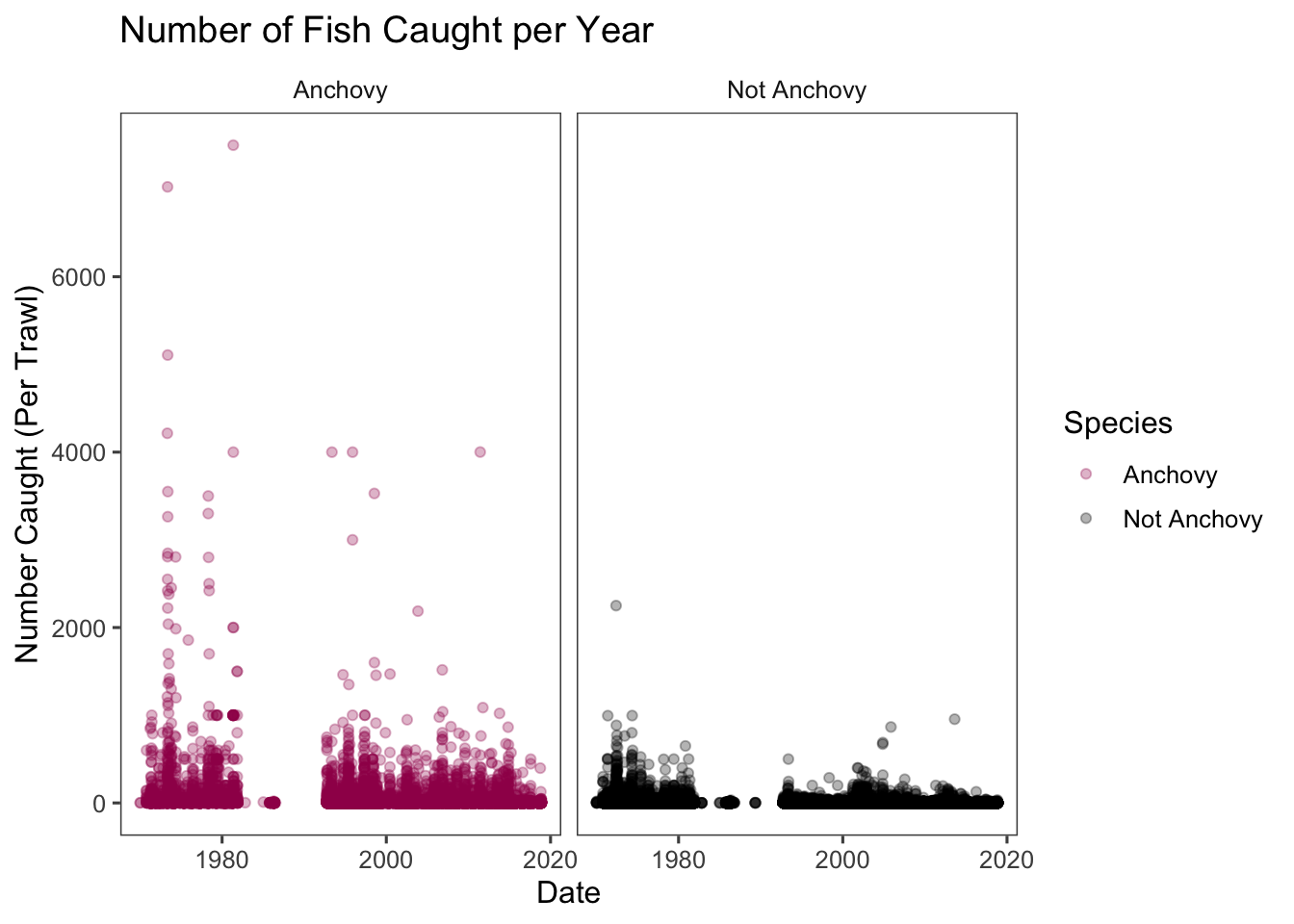
Here is a plot of the catch based on date with anchovies colored Pink as to get an idea of what the data looks like.

Code

library(patchwork)


Attaching package: 'patchwork'

The following object is masked from 'package:MASS':

    area

Code

catch_plot <- catch_clean %>% 
  mutate(date = dmy(date)) 


catch_plot$species_group <- ifelse(catch_plot$species_code == "NA",
                                   "Anchovy",
                                   "Not Anchovy")

ggplot(catch_plot, aes(x = date, y = number,
                       color = species_group)) +
  geom_point(alpha = .3) +
  ggthemes::theme_few()+
  labs(x = "Date",
       y = "Number Caught (Per Trawl)",
       title = "Number of Fish Caught per Year",
       color = "Species") +
  scale_color_manual(values = c("Not Anchovy" = "black",
                                "Anchovy" = "#A0185A"))+
  facet_wrap(~species_group)

In this plot we can see that we catch Anchovies at a much higher quantity per trawl as well as over time. The bottom plots show a smaller date range so we can see peaks in Anchovies that are not as apparent in other species. There are some sampling gaps that become apparent in 1984 as well as 1988, with much fewer observations in general in the 80’s. This may result in less representative data.

Preliminary analysis: Indicator species

Indicator species:

reflect the biotic or abiotic state of the environment;
provide evidence for the impacts of environmental change; or
predict the diversity of other species, taxa or communities within a area group

By comparing Anchovy population to that of indicator species, it may shed light on whether Anchovy population can be representative of the indicator. We will be performing analyses on the four locales apparent in the bay as the indicator analysis is predicated on the fact the indicator species indicates the area group it is in.

To perform the indicator species analysis we will be using the function multipatt from the package indispecies. The function takes a group vector and a species matrix

Code

indicator <- catch_clean %>% 
  dplyr::select(catch_info_trawl_id, species_code, number, locale) %>% 
  pivot_wider(names_from = species_code, values_from = number, values_fn = sum) %>% 
  mutate(across(where(is.numeric), ~replace_na(., 0))) %>% 
  filter(!locale == 'BLANK')

group_vector <- indicator$locale

species_matrix <- as.matrix(indicator[, -c(1, 2)])

Now we can run the function multipatt to find indicator species values for our groups

Code

indval <- multipatt(species_matrix, group_vector, 
                    control = how(nperm=999))

Code

summary(indval, alpha = .1)


 Multilevel pattern analysis
 ---------------------------

 Association function: IndVal.g
 Significance level (alpha): 0.1

 Total number of species: 162
 Selected number of species: 50 
 Number of species associated to 1 group: 33 
 Number of species associated to 2 groups: 12 
 Number of species associated to 3 groups: 5 

 List of species associated to each combination: 

 Group CENTRAL BAY  #sps.  13 
     stat p.value   
SSD 0.456   0.009 **
CLF 0.217   0.039 * 
POM 0.110   0.027 * 
ps  0.066   0.051 . 
HH  0.065   0.065 . 
CRL 0.065   0.073 . 
OP  0.059   0.046 * 
JM  0.059   0.037 * 
BSC 0.050   0.045 * 
es  0.046   0.086 . 
IRL 0.042   0.032 * 
ssd 0.042   0.025 * 
PB  0.039   0.090 . 

 Group SAN PABLO BAY  #sps.  4 
     stat p.value  
BR  0.449   0.012 *
DT  0.328   0.048 *
TS  0.277   0.025 *
BSK 0.214   0.053 .

 Group SOUTH BAY  #sps.  2 
     stat p.value  
CT  0.308   0.072 .
DSP 0.285   0.091 .

 Group SUISUN BAY  #sps.  14 
     stat p.value    
SB  0.880   0.001 ***
SF  0.768   0.001 ***
TFS 0.417   0.001 ***
SST 0.303   0.001 ***
DLS 0.204   0.007 ** 
BDG 0.204   0.005 ** 
TP  0.148   0.017 *  
CC  0.129   0.004 ** 
BLP 0.129   0.005 ** 
CK  0.091   0.013 *  
KS  0.091   0.020 *  
DS  0.089   0.016 *  
BBC 0.088   0.017 *  
PL  0.086   0.053 .  

 Group CENTRAL BAY+SAN PABLO BAY  #sps.  6 
     stat p.value    
PMS 0.652   0.001 ***
PH  0.535   0.002 ** 
BG  0.495   0.001 ***
BPF 0.338   0.015 *  
WSP 0.320   0.012 *  
BHS 0.225   0.069 .  

 Group CENTRAL BAY+SOUTH BAY  #sps.  1 
    stat p.value  
SD 0.381   0.039 *

 Group CENTRAL BAY+SUISUN BAY  #sps.  1 
    stat p.value  
PS 0.267   0.053 .

 Group SAN PABLO BAY+SOUTH BAY  #sps.  1 
    stat p.value  
BS 0.343   0.048 *

 Group SAN PABLO BAY+SUISUN BAY  #sps.  2 
     stat p.value    
YG  0.574   0.001 ***
LFS 0.538   0.001 ***

 Group SOUTH BAY+SUISUN BAY  #sps.  1 
   stat p.value  
UG 0.32    0.07 .

 Group CENTRAL BAY+SAN PABLO BAY+SOUTH BAY  #sps.  3 
     stat p.value    
NA  0.811   0.001 ***
SSP 0.762   0.003 ** 
WC  0.385   0.034 *  

 Group CENTRAL BAY+SAN PABLO BAY+SUISUN BAY  #sps.  1 
     stat p.value    
PSD 0.527   0.001 ***

 Group SAN PABLO BAY+SOUTH BAY+SUISUN BAY  #sps.  1 
    stat p.value  
LS 0.353   0.028 *
---
Signif. codes:  0 '***' 0.001 '**' 0.01 '*' 0.05 '.' 0.1 ' ' 1

The output of that looks pretty bad, and the function does not let you pull out different pieces without the P-values changing so I made this reference table of the top 2 species in each singular group.

Code

ind_table <- data.frame(
  Species = c(
    "SSD", "CLF",        # CENTRAL BAY top 2
    "BR", "DT",          # SAN PABLO BAY top 2
    "CT", "DSP",         # SOUTH BAY top 2
    "SB", "SF"           # SUISUN BAY top 2
  ),
  Group = c(
    rep("CENTRAL BAY", 2),
    rep("SAN PABLO BAY", 2),
    rep("SOUTH BAY", 2),
    rep("SUISUN BAY", 2)
  ),
  Stat = c(
    0.456, 0.217,        # CENTRAL BAY
    0.449, 0.328,        # SAN PABLO BAY
    0.308, 0.285,        # SOUTH BAY
    0.880, 0.768         # SUISUN BAY
  ),
  'P_Value' = c(
    0.008, 0.044,        # CENTRAL BAY
    0.009, 0.051,        # SAN PABLO BAY
    0.072, 0.077,        # SOUTH BAY
    0.001, 0.001         # SUISUN BAY
  )
) 
  
ind_table %>% 
  kable( format = "html", digits = 3,
      caption = "Top 2 indicator species in each region ") %>% 
  kable_styling(
    bootstrap_options = c("striped", "hover", "condensed", "responsive"),
    full_width = FALSE,
    position   = "center",
    font_size  = 14
  ) %>% 
  row_spec(0, bold = TRUE, color = "white", background = "#A0185A") %>%  # header
  row_spec(1:nrow(ind_table), color = "black", background = "#FFC4EB") %>% 
  scroll_box(width = "300px", height = "400px")

Top 2 indicator species in each region
Species	Group	Stat	P_Value
SSD	CENTRAL BAY	0.456	0.008
CLF	CENTRAL BAY	0.217	0.044
BR	SAN PABLO BAY	0.449	0.009
DT	SAN PABLO BAY	0.328	0.051
CT	SOUTH BAY	0.308	0.072
DSP	SOUTH BAY	0.285	0.077
SB	SUISUN BAY	0.880	0.001
SF	SUISUN BAY	0.768	0.001

From the summary we can see that the top species for the four San Francisco Bay locales are:

Group CENTRAL BAY SSD: Speckled Sanddab

Group SAN PABLO BAY BR: Bat Ray

Group SOUTH BAY CT: California Tonguefish

Group SUISUN BAY SB: Striped Bass

Next we are going to compare Northern Anchovy catches to these species using a hurdle model

Hurdle model and create function

Hurdle Models are a class of models for count data that help handle excess zeros and over dispersion, which fits our data nicely. It handles these by treating presence as a binary operator (present vs not present) and running a binomial(link = ‘logit’) model. The model also includes abundance, which analyzes count data using a negative binomial model.

Presence: \[ \begin{align} \text{Presence} &\sim Binomial(1, p) \\ logit(p) &= \beta_0 + \beta_1 \text{NorthernAnchovyZ}* \beta_2 \text{inregion} \end{align} \] Abundance: \[ \begin{align} \text{Abundance} &\sim NegBin(\lambda, \theta) \\ log(\lambda) &= \beta_0 + \beta_1 \text{NorthernAnchovyZ}* \beta_2 \text{inregion} \end{align} \]

If we can use Northern Anchovy as a predictor for indicator species, we would expect both

Assumption: \[ \begin{align} \ H_0 = \beta_1presence = 0 \\ \ H_0 = \beta_1abundance = 0 \\ \ H_A = \beta_1presence \ne 0\\ \ H_A = \beta_1abundance \ne 0\\ \end{align} \]

We use the z-score transformed count of Northern Anchovy as it:

Helps with numerical stability, especially in interaction terms
Is useful when comparing effect sizes across variables on different scales

Simulate data

Before we use this model we will be simulating data in an attempt to see if the model is appropriate for our data.

Code

set.seed(42)

n_sim <- 1000

# Predictor: standardized anchovy index
northern_anchovy_z <- rnorm(n_sim, mean = 0, sd = 1)

# in_region (TRUE/FALSE)
in_region <- rep(c(TRUE, FALSE), length.out = n_sim)

# Logistic (presence/absence)
beta0_presence <- -0.5
beta1_presence <-  1.2
beta_region_presence <- 0.5              
beta_interaction_presence <- -0.3        

# Abundance (given present)
beta0_abundance <- 0.7
beta1_abundance <- 0.4
beta_region_abundance <- -0.6            
beta_interaction_abundance <- 0.2        

theta <- 1.8  # NB dispersion

# Probability of presence *including region + interaction*
linpred_presence <- beta0_presence +
  beta1_presence * northern_anchovy_z +
  beta_region_presence * in_region +
  beta_interaction_presence * northern_anchovy_z * in_region

p_presence <- plogis(linpred_presence)

# Storage
presence  <- rep(0, n_sim)
abundance <- rep(0, n_sim)

for (i in 1:n_sim) {

  presence[i] <- rbinom(1, 1, p_presence[i])

  if (presence[i] == 1) {

    # abundance linear predictor
    linpred_abundance <- beta0_abundance +
      beta1_abundance * northern_anchovy_z[i] +
      beta_region_abundance * in_region[i] +
      beta_interaction_abundance * northern_anchovy_z[i] * in_region[i]

    lambda_i <- exp(linpred_abundance)

    repeat {
      y <- rnbinom(1, mu = lambda_i, size = theta)
      if (y > 0) {
        abundance[i] <- y
        break
      }
    }
  }
}

sim_data <- tibble(
  northern_anchovy_z,
  in_region,
  presence,
  abundance
)

Model Simulated data

Code

m1 <- glm(presence ~ northern_anchovy_z * in_region, 
          data = sim_data, 
          family = binomial(link = 'logit'))

m2 <- glm.nb(abundance ~ northern_anchovy_z * in_region, 
             data = sim_data)

m1_tidy <- tidy(m1)%>% 
  mutate(model = "Presence (Logit)")
m2_tidy <- tidy(m2)%>% 
  mutate(model = "Abundance (NegBin)")

# combine and format
all_models <- bind_rows(m1_tidy, m2_tidy) %>%
  dplyr::select(model, term, estimate, std.error, statistic, p.value)%>%
  rename(
    Model = model,
    Term = term,
    Estimate = estimate,
    SE = std.error,
    'Test Stat' = statistic,
    'P-Value'   = p.value
  ) 

kable(all_models, format = "html", digits = 3,
      caption = "Joint Model Output: Presence vs Abundance")%>%
  kable_styling(
    bootstrap_options = c("striped", "hover", "condensed", "responsive"),
    full_width = FALSE,
    position   = "center",
    font_size  = 14
  ) %>% 
  row_spec(0, bold = TRUE, color = "white", background = "#A0185A") %>%  # header
  row_spec(1:nrow(all_models), color = "black", background = "#FFC4EB")  # body rows

Joint Model Output: Presence vs Abundance
Model	Term	Estimate	SE	Test Stat	P-Value
Presence (Logit)	(Intercept)	-0.277	0.103	-2.690	0.007
Presence (Logit)	northern_anchovy_z	1.233	0.132	9.362	0.000
Presence (Logit)	in_regionTRUE	0.212	0.141	1.508	0.131
Presence (Logit)	northern_anchovy_z:in_regionTRUE	-0.388	0.172	-2.260	0.024
Abundance (NegBin)	(Intercept)	0.025	0.072	0.345	0.730
Abundance (NegBin)	northern_anchovy_z	0.972	0.072	13.463	0.000
Abundance (NegBin)	in_regionTRUE	-0.045	0.100	-0.449	0.653
Abundance (NegBin)	northern_anchovy_z:in_regionTRUE	-0.251	0.102	-2.464	0.014

That looks great! Our values for the parameters were returned!

Because we are running and fitting this model four times, it sounds like I should make it into a function

Function

Code

#' predict indicator
#' @param df
#' Data frame used for analysis
#' @param sp_code 
#' Species code (wrapped in '')
#' @param region 
#' Locale (all capitals wrapped in '')
#' @returns
#' a list containing: 
#' summary_table 
#' pred_pres_table
#'  pred_abu_table 
#'  combined_table 
#'  stage1_pred 
#'  stage2_pred
#'  combined_pred 
#'  plot 
#' @export
#'
#' @examples
predict_indicator <- function(df, sp_code, region) {

  species_name <- species_key_clean %>% 
    filter(species_code == sp_code) %>% 
    pull(species_name) %>% 
    make_clean_names()

  catch_plot <- df %>% 
    filter(species_code == 'NA' | species_code == sp_code) %>% 
    mutate(in_region = ifelse(locale == region, TRUE, FALSE)) %>% 
    group_by(species_code, catch_info_trawl_id, in_region) %>% 
    summarize(count = sum(number), .groups = "drop") %>% 
    pivot_wider(names_from = species_code,
                values_from = count) %>% 
    set_names(c('trawl_id', 'in_region', 'northern_anchovy', species_name)) 

  catch_plot[is.na(catch_plot)] <- 0

  a <- mean(catch_plot$northern_anchovy)
  b <- sd(catch_plot$northern_anchovy)

  catch_plot <- catch_plot %>% 
    mutate(
      northern_anchovy_z = (northern_anchovy - a) / b,
      presence = ifelse(.data[[species_name]] > 0, 1, 0),
      abundance = ifelse(.data[[species_name]] > 0, .data[[species_name]], NA)
    )

  # Stage 1 & 2 models
  m1 <- glm(presence ~ northern_anchovy_z * in_region, data = catch_plot, family = binomial(link = 'logit'))
  m2 <- glm.nb(abundance ~ northern_anchovy_z * in_region, data = catch_plot)

  # Tidy outputs
  m1_tidy <- tidy(m1) %>% mutate(model = "Presence (Logit)")
  m2_tidy <- tidy(m2) %>% mutate(model = "Abundance (NegBin)")

  all_models <- bind_rows(m1_tidy, m2_tidy) %>%
    dplyr::select(model, term, estimate, std.error, statistic, p.value) %>%
    rename(
      Model = model,
      Term = term,
      Estimate = estimate,
      SE = std.error,
      'Test Stat' = statistic,
      'P-Value' = p.value
    )

  # Styled kable for model summary
  summary_table <- all_models %>% 
    kable(format = "html", digits = 3, caption = "Joint Model Output: Presence vs Abundance") %>% 
    kable_styling(
      bootstrap_options = c("striped", "hover", "condensed", "responsive"),
      full_width = FALSE,
      position = "center",
      font_size = 14
    ) %>% 
    row_spec(0, bold = TRUE, color = "white", background = "#A0185A") %>% 
    row_spec(1:nrow(all_models), color = "black", background = "#FFC4EB")

  # Prediction grid
  grid_data <- expand_grid(
    in_region = c(TRUE, FALSE),
    northern_anchovy_z = seq(min(catch_plot$northern_anchovy_z), max(catch_plot$northern_anchovy_z), by = 1)
  )

  # Predictions
  predict_pres <- predict(m1, newdata = grid_data, type = "link", se.fit = TRUE)
  predict_abu  <- predict(m2, newdata = grid_data, type = "link", se.fit = TRUE)

  pred_pres_result <- grid_data %>% 
    mutate(
      fit_link = predict_pres$fit,
      se = predict_pres$se.fit,
      pred_tbs = plogis(fit_link),
      lower = plogis(fit_link - 1.96*se),
      upper = plogis(fit_link + 1.96*se)
    )

  pred_abu_result <- grid_data %>% 
    mutate(
      fit_link = predict_abu$fit,
      se = predict_abu$se.fit,
      pred_tbs = exp(fit_link),
      lower = exp(fit_link - 1.96*se),
      upper = exp(fit_link + 1.96*se)
    )

  # Merge predictions
  combined_pred <- pred_pres_result %>% 
    mutate(
      expected_count = pred_tbs * pred_abu_result$pred_tbs,
      lower_expected = lower * pred_abu_result$lower,
      upper_expected = upper * pred_abu_result$upper
    )

  # Styled kables for predictions
  pred_pres_table <- pred_pres_result %>% 
    kable(format = "html", digits = 3, caption = "Presence Predictions") %>% 
    kable_styling(
      bootstrap_options = c("striped", "hover", "condensed", "responsive"),
      full_width = FALSE,
      position = "center",
      font_size = 14
    ) %>% 
    row_spec(0, bold = TRUE, color = "white", background = "#A0185A") %>% 
    row_spec(1:nrow(pred_pres_result), color = "black", background = "#FFC4EB") %>% 
    scroll_box(width = "800px", height = "300px")

  pred_abu_table <- pred_abu_result %>% 
    kable(format = "html", digits = 3, caption = "Abundance Predictions") %>% 
    kable_styling(
      bootstrap_options = c("striped", "hover", "condensed", "responsive"),
      full_width = FALSE,
      position = "center",
      font_size = 14
    ) %>% 
    row_spec(0, bold = TRUE, color = "white", background = "#A0185A") %>% 
    row_spec(1:nrow(pred_abu_result), color = "black", background = "#FFC4EB") %>% 
    scroll_box(width = "800px", height = "300px")

  combined_table <- combined_pred %>% 
    kable(format = "html", digits = 3, caption = "Expected Counts (Presence × Abundance)") %>% 
    kable_styling(
      bootstrap_options = c("striped", "hover", "condensed", "responsive"),
      full_width = FALSE,
      position = "center",
      font_size = 14
    ) %>% 
    row_spec(0, bold = TRUE, color = "white", background = "#A0185A") %>% 
    row_spec(1:nrow(combined_pred), color = "black", background = "#FFC4EB") %>% 
    scroll_box(width = "800px", height = "300px")

  # Plot
  plot <- ggplot(combined_pred, aes(northern_anchovy_z, expected_count)) +
    facet_wrap(~in_region,
               labeller = as_labeller(c(`TRUE` = "In Region", `FALSE` = "Outside Region"))) +
    geom_line(color = '#A0185A') +
    geom_ribbon(aes(ymin = lower_expected, ymax = upper_expected),
                alpha = .3, fill = '#ABC798') +
    labs(x = 'Northern Anchovy Z',
         y = str_to_title(str_replace_all(species_name, "_", " "))) +
    theme_clean()

  return(list(
    summary_table = summary_table,
    pred_pres_table = pred_pres_table,
    pred_abu_table = pred_abu_table,
    combined_table = combined_table,
    stage1_pred = pred_pres_result,
    stage2_pred = pred_abu_result,
    combined_pred = combined_pred,
    plot = plot
  ))
}

Function Call: Central Bay

The top indicator for the Central Bay was the Speckled Sanddab so we can call the function for that species and region

Code

speckled <- predict_indicator(catch_clean, 'SSD', 'CENTRAL BAY')

Now speckled is encoded with our model summaries, predictions, and plot. For this I will show all outputs, in later chunks I will bypass showing predictions

Model Summary

Code

speckled$summary_table

Joint Model Output: Presence vs Abundance
Model	Term	Estimate	SE	Test Stat	P-Value
Presence (Logit)	(Intercept)	-1.556	0.031	-49.769	0.000
Presence (Logit)	northern_anchovy_z	-0.531	0.087	-6.127	0.000
Presence (Logit)	in_regionTRUE	1.089	0.081	13.490	0.000
Presence (Logit)	northern_anchovy_z:in_regionTRUE	0.160	0.172	0.931	0.352
Abundance (NegBin)	(Intercept)	1.965	0.033	59.284	0.000
Abundance (NegBin)	northern_anchovy_z	-0.058	0.053	-1.082	0.279
Abundance (NegBin)	in_regionTRUE	0.816	0.077	10.546	0.000
Abundance (NegBin)	northern_anchovy_z:in_regionTRUE	-0.101	0.145	-0.696	0.487

Coefficient discussion

Each coefficient table will have 8 estimates and p-values. The first 4 refer to the Presence (logit) model, the second 4 refer to the Abundance (negbin) model. Each of the models have the same structure as well: intercept, northern_anchovy_z, in_regionTRUE, and northern_anchovy_z:in_regionTRUE. The intercept is set at the level in_regionFalse, meaning its the outcome of not being in the indicators region, and not having Anchovies present. Northern_anchovy_z estimate and p_value show the effect on Northern_anchovy_z outside the region. In_regionTRUE estimate and p_value show the effect of being in the the region on the indicator Presence and Abundance. Lastly northern_anchovy_z:in_regionTRUE shows the interaction between northern anchovies and being inside an indicators region.

Presence Prediction

Code

speckled$pred_pres_table

Presence Predictions
in_region	northern_anchovy_z	fit_link	se	pred_tbs	lower	upper
TRUE	-0.273	-0.367	0.083	0.409	0.371	0.449
TRUE	0.727	-0.737	0.134	0.324	0.269	0.384
TRUE	1.727	-1.107	0.271	0.248	0.163	0.360
TRUE	2.727	-1.477	0.417	0.186	0.092	0.341
TRUE	3.727	-1.847	0.564	0.136	0.050	0.323
TRUE	4.727	-2.217	0.712	0.098	0.026	0.305
TRUE	5.727	-2.587	0.860	0.070	0.014	0.289
TRUE	6.727	-2.958	1.009	0.049	0.007	0.273
TRUE	7.727	-3.328	1.157	0.035	0.004	0.257
TRUE	8.727	-3.698	1.306	0.024	0.002	0.243
TRUE	9.727	-4.068	1.455	0.017	0.001	0.228
TRUE	10.727	-4.438	1.603	0.012	0.001	0.215
TRUE	11.727	-4.808	1.752	0.008	0.000	0.202
TRUE	12.727	-5.178	1.901	0.006	0.000	0.190
TRUE	13.727	-5.549	2.050	0.004	0.000	0.178
TRUE	14.727	-5.919	2.199	0.003	0.000	0.167
TRUE	15.727	-6.289	2.348	0.002	0.000	0.156
TRUE	16.727	-6.659	2.497	0.001	0.000	0.146
TRUE	17.727	-7.029	2.645	0.001	0.000	0.137
TRUE	18.727	-7.399	2.794	0.001	0.000	0.128
TRUE	19.727	-7.770	2.943	0.000	0.000	0.119
TRUE	20.727	-8.140	3.092	0.000	0.000	0.111
TRUE	21.727	-8.510	3.241	0.000	0.000	0.104
TRUE	22.727	-8.880	3.390	0.000	0.000	0.097
TRUE	23.727	-9.250	3.539	0.000	0.000	0.090
TRUE	24.727	-9.620	3.688	0.000	0.000	0.084
TRUE	25.727	-9.990	3.837	0.000	0.000	0.078
TRUE	26.727	-10.361	3.986	0.000	0.000	0.073
TRUE	27.727	-10.731	4.135	0.000	0.000	0.067
FALSE	-0.273	-1.412	0.032	0.196	0.186	0.206
FALSE	0.727	-1.942	0.080	0.125	0.109	0.144
FALSE	1.727	-2.473	0.164	0.078	0.058	0.104
FALSE	2.727	-3.004	0.249	0.047	0.030	0.075
FALSE	3.727	-3.534	0.336	0.028	0.015	0.053
FALSE	4.727	-4.065	0.422	0.017	0.007	0.038
FALSE	5.727	-4.595	0.508	0.010	0.004	0.027
FALSE	6.727	-5.126	0.595	0.006	0.002	0.019
FALSE	7.727	-5.657	0.681	0.003	0.001	0.013
FALSE	8.727	-6.187	0.768	0.002	0.000	0.009
FALSE	9.727	-6.718	0.854	0.001	0.000	0.006
FALSE	10.727	-7.248	0.941	0.001	0.000	0.004
FALSE	11.727	-7.779	1.028	0.000	0.000	0.003
FALSE	12.727	-8.310	1.114	0.000	0.000	0.002
FALSE	13.727	-8.840	1.201	0.000	0.000	0.002
FALSE	14.727	-9.371	1.287	0.000	0.000	0.001
FALSE	15.727	-9.901	1.374	0.000	0.000	0.001
FALSE	16.727	-10.432	1.460	0.000	0.000	0.001
FALSE	17.727	-10.963	1.547	0.000	0.000	0.000
FALSE	18.727	-11.493	1.634	0.000	0.000	0.000
FALSE	19.727	-12.024	1.720	0.000	0.000	0.000
FALSE	20.727	-12.554	1.807	0.000	0.000	0.000
FALSE	21.727	-13.085	1.893	0.000	0.000	0.000
FALSE	22.727	-13.616	1.980	0.000	0.000	0.000
FALSE	23.727	-14.146	2.067	0.000	0.000	0.000
FALSE	24.727	-14.677	2.153	0.000	0.000	0.000
FALSE	25.727	-15.207	2.240	0.000	0.000	0.000
FALSE	26.727	-15.738	2.326	0.000	0.000	0.000
FALSE	27.727	-16.269	2.413	0.000	0.000	0.000

Abundance Prediction

Code

speckled$pred_abu_table

Abundance Predictions
in_region	northern_anchovy_z	fit_link	se	pred_tbs	lower	upper
TRUE	-0.273	2.825	0.076	16.854	14.533	19.545
TRUE	0.727	2.666	0.126	14.380	11.227	18.419
TRUE	1.727	2.507	0.250	12.270	7.512	20.043
TRUE	2.727	2.348	0.382	10.469	4.952	22.134
TRUE	3.727	2.190	0.515	8.933	3.253	24.531
TRUE	4.727	2.031	0.649	7.622	2.134	27.223
TRUE	5.727	1.872	0.784	6.504	1.399	30.231
TRUE	6.727	1.714	0.919	5.549	0.917	33.583
TRUE	7.727	1.555	1.053	4.735	0.601	37.316
TRUE	8.727	1.396	1.188	4.040	0.394	41.470
TRUE	9.727	1.238	1.323	3.447	0.258	46.091
TRUE	10.727	1.079	1.458	2.941	0.169	51.231
TRUE	11.727	0.920	1.593	2.510	0.111	56.947
TRUE	12.727	0.761	1.728	2.141	0.072	63.304
TRUE	13.727	0.603	1.863	1.827	0.047	70.373
TRUE	14.727	0.444	1.998	1.559	0.031	78.234
TRUE	15.727	0.285	2.133	1.330	0.020	86.974
TRUE	16.727	0.127	2.268	1.135	0.013	96.692
TRUE	17.727	-0.032	2.403	0.968	0.009	107.498
TRUE	18.727	-0.191	2.538	0.826	0.006	119.513
TRUE	19.727	-0.349	2.673	0.705	0.004	132.873
TRUE	20.727	-0.508	2.808	0.602	0.002	147.727
TRUE	21.727	-0.667	2.943	0.513	0.002	164.243
TRUE	22.727	-0.826	3.078	0.438	0.001	182.607
TRUE	23.727	-0.984	3.213	0.374	0.001	203.025
TRUE	24.727	-1.143	3.348	0.319	0.000	225.727
TRUE	25.727	-1.302	3.483	0.272	0.000	250.969
TRUE	26.727	-1.460	3.618	0.232	0.000	279.035
TRUE	27.727	-1.619	3.753	0.198	0.000	310.241
FALSE	-0.273	1.981	0.033	7.251	6.797	7.736
FALSE	0.727	1.923	0.056	6.845	6.127	7.646
FALSE	1.727	1.866	0.105	6.461	5.262	7.934
FALSE	2.727	1.808	0.156	6.099	4.490	8.286
FALSE	3.727	1.750	0.209	5.757	3.824	8.669
FALSE	4.727	1.693	0.262	5.435	3.255	9.075
FALSE	5.727	1.635	0.315	5.130	2.770	9.503
FALSE	6.727	1.577	0.368	4.843	2.356	9.954
FALSE	7.727	1.520	0.421	4.571	2.004	10.427
FALSE	8.727	1.462	0.474	4.315	1.705	10.924
FALSE	9.727	1.404	0.527	4.073	1.450	11.445
FALSE	10.727	1.347	0.580	3.845	1.233	11.991
FALSE	11.727	1.289	0.633	3.630	1.049	12.564
FALSE	12.727	1.231	0.687	3.426	0.892	13.164
FALSE	13.727	1.174	0.740	3.234	0.758	13.793
FALSE	14.727	1.116	0.793	3.053	0.645	14.453
FALSE	15.727	1.058	0.846	2.882	0.548	15.144
FALSE	16.727	1.001	0.900	2.721	0.466	15.868
FALSE	17.727	0.943	0.953	2.568	0.397	16.627
FALSE	18.727	0.885	1.006	2.424	0.337	17.423
FALSE	19.727	0.828	1.060	2.288	0.287	18.257
FALSE	20.727	0.770	1.113	2.160	0.244	19.131
FALSE	21.727	0.712	1.166	2.039	0.207	20.047
FALSE	22.727	0.655	1.219	1.925	0.176	21.006
FALSE	23.727	0.597	1.273	1.817	0.150	22.012
FALSE	24.727	0.539	1.326	1.715	0.128	23.066
FALSE	25.727	0.482	1.379	1.619	0.108	24.170
FALSE	26.727	0.424	1.433	1.528	0.092	25.328
FALSE	27.727	0.366	1.486	1.443	0.078	26.541

Combined Prediction

Code

speckled$combined_table

Expected Counts (Presence × Abundance)
in_region	northern_anchovy_z	fit_link	se	pred_tbs	lower	upper	expected_count	lower_expected	upper_expected
TRUE	-0.273	-0.367	0.083	0.409	0.371	0.449	6.900	5.387	8.780
TRUE	0.727	-0.737	0.134	0.324	0.269	0.384	4.655	3.019	7.070
TRUE	1.727	-1.107	0.271	0.248	0.163	0.360	3.049	1.222	7.217
TRUE	2.727	-1.477	0.417	0.186	0.092	0.341	1.946	0.454	7.540
TRUE	3.727	-1.847	0.564	0.136	0.050	0.323	1.217	0.161	7.913
TRUE	4.727	-2.217	0.712	0.098	0.026	0.305	0.749	0.056	8.311
TRUE	5.727	-2.587	0.860	0.070	0.014	0.289	0.455	0.019	8.727
TRUE	6.727	-2.958	1.009	0.049	0.007	0.273	0.274	0.007	9.159
TRUE	7.727	-3.328	1.157	0.035	0.004	0.257	0.164	0.002	9.604
TRUE	8.727	-3.698	1.306	0.024	0.002	0.243	0.098	0.001	10.061
TRUE	9.727	-4.068	1.455	0.017	0.001	0.228	0.058	0.000	10.530
TRUE	10.727	-4.438	1.603	0.012	0.001	0.215	0.034	0.000	11.010
TRUE	11.727	-4.808	1.752	0.008	0.000	0.202	0.020	0.000	11.501
TRUE	12.727	-5.178	1.901	0.006	0.000	0.190	0.012	0.000	12.004
TRUE	13.727	-5.549	2.050	0.004	0.000	0.178	0.007	0.000	12.517
TRUE	14.727	-5.919	2.199	0.003	0.000	0.167	0.004	0.000	13.041
TRUE	15.727	-6.289	2.348	0.002	0.000	0.156	0.002	0.000	13.576
TRUE	16.727	-6.659	2.497	0.001	0.000	0.146	0.001	0.000	14.122
TRUE	17.727	-7.029	2.645	0.001	0.000	0.137	0.001	0.000	14.680
TRUE	18.727	-7.399	2.794	0.001	0.000	0.128	0.001	0.000	15.248
TRUE	19.727	-7.770	2.943	0.000	0.000	0.119	0.000	0.000	15.828
TRUE	20.727	-8.140	3.092	0.000	0.000	0.111	0.000	0.000	16.420
TRUE	21.727	-8.510	3.241	0.000	0.000	0.104	0.000	0.000	17.024
TRUE	22.727	-8.880	3.390	0.000	0.000	0.097	0.000	0.000	17.640
TRUE	23.727	-9.250	3.539	0.000	0.000	0.090	0.000	0.000	18.269
TRUE	24.727	-9.620	3.688	0.000	0.000	0.084	0.000	0.000	18.912
TRUE	25.727	-9.990	3.837	0.000	0.000	0.078	0.000	0.000	19.567
TRUE	26.727	-10.361	3.986	0.000	0.000	0.073	0.000	0.000	20.237
TRUE	27.727	-10.731	4.135	0.000	0.000	0.067	0.000	0.000	20.922
FALSE	-0.273	-1.412	0.032	0.196	0.186	0.206	1.421	1.267	1.593
FALSE	0.727	-1.942	0.080	0.125	0.109	0.144	0.858	0.669	1.098
FALSE	1.727	-2.473	0.164	0.078	0.058	0.104	0.503	0.303	0.826
FALSE	2.727	-3.004	0.249	0.047	0.030	0.075	0.288	0.133	0.620
FALSE	3.727	-3.534	0.336	0.028	0.015	0.053	0.163	0.057	0.462
FALSE	4.727	-4.065	0.422	0.017	0.007	0.038	0.092	0.024	0.343
FALSE	5.727	-4.595	0.508	0.010	0.004	0.027	0.051	0.010	0.253
FALSE	6.727	-5.126	0.595	0.006	0.002	0.019	0.029	0.004	0.186
FALSE	7.727	-5.657	0.681	0.003	0.001	0.013	0.016	0.002	0.137
FALSE	8.727	-6.187	0.768	0.002	0.000	0.009	0.009	0.001	0.100
FALSE	9.727	-6.718	0.854	0.001	0.000	0.006	0.005	0.000	0.073
FALSE	10.727	-7.248	0.941	0.001	0.000	0.004	0.003	0.000	0.054
FALSE	11.727	-7.779	1.028	0.000	0.000	0.003	0.002	0.000	0.039
FALSE	12.727	-8.310	1.114	0.000	0.000	0.002	0.001	0.000	0.029
FALSE	13.727	-8.840	1.201	0.000	0.000	0.002	0.000	0.000	0.021
FALSE	14.727	-9.371	1.287	0.000	0.000	0.001	0.000	0.000	0.015
FALSE	15.727	-9.901	1.374	0.000	0.000	0.001	0.000	0.000	0.011
FALSE	16.727	-10.432	1.460	0.000	0.000	0.001	0.000	0.000	0.008
FALSE	17.727	-10.963	1.547	0.000	0.000	0.000	0.000	0.000	0.006
FALSE	18.727	-11.493	1.634	0.000	0.000	0.000	0.000	0.000	0.004
FALSE	19.727	-12.024	1.720	0.000	0.000	0.000	0.000	0.000	0.003
FALSE	20.727	-12.554	1.807	0.000	0.000	0.000	0.000	0.000	0.002
FALSE	21.727	-13.085	1.893	0.000	0.000	0.000	0.000	0.000	0.002
FALSE	22.727	-13.616	1.980	0.000	0.000	0.000	0.000	0.000	0.001
FALSE	23.727	-14.146	2.067	0.000	0.000	0.000	0.000	0.000	0.001
FALSE	24.727	-14.677	2.153	0.000	0.000	0.000	0.000	0.000	0.001
FALSE	25.727	-15.207	2.240	0.000	0.000	0.000	0.000	0.000	0.000
FALSE	26.727	-15.738	2.326	0.000	0.000	0.000	0.000	0.000	0.000
FALSE	27.727	-16.269	2.413	0.000	0.000	0.000	0.000	0.000	0.000

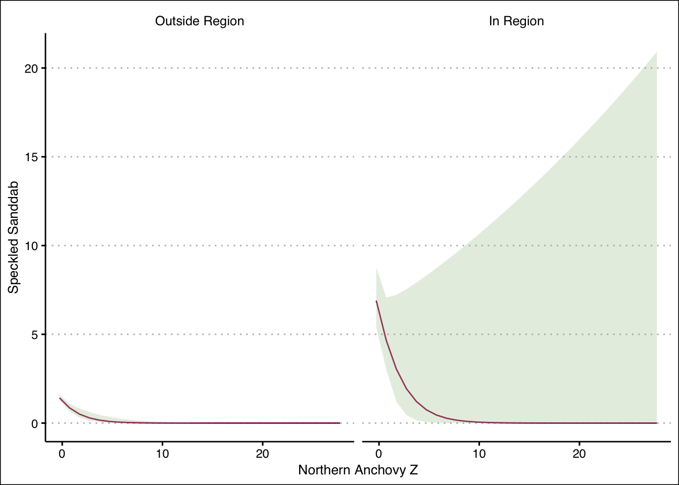
Speckled plot

Code

speckled$plot

Discussion: Speckled Sanddab

Based on the function we can see significance in presence of Anchovy and the region in both presence and abundance. This indicates that the presence of Anchovy comes at the cost of presence of Sanddabs. This model does not seem to fit incredibly well when looking at the plot, which can be seen by the flat lines and giant confidence intervals.

Function Call: San Pablo Bay

Code

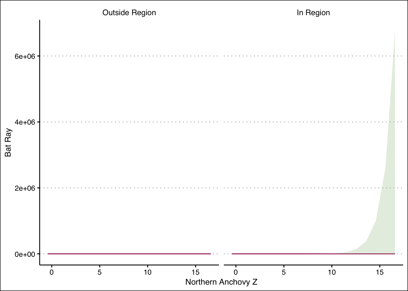
bat_ray <- predict_indicator(catch_clean, 'BR', 'SAN PABLO BAY')

Model Summary

Code

bat_ray$summary_table

Joint Model Output: Presence vs Abundance
Model	Term	Estimate	SE	Test Stat	P-Value
Presence (Logit)	(Intercept)	2.598	0.043	59.788	0.000
Presence (Logit)	northern_anchovy_z	-0.801	0.034	-23.834	0.000
Presence (Logit)	in_regionTRUE	-1.980	0.960	-2.063	0.039
Presence (Logit)	northern_anchovy_z:in_regionTRUE	1.476	0.932	1.584	0.113
Abundance (NegBin)	(Intercept)	4.321	0.018	236.057	0.000
Abundance (NegBin)	northern_anchovy_z	-0.223	0.022	-10.216	0.000
Abundance (NegBin)	in_regionTRUE	-3.409	0.917	-3.719	0.000
Abundance (NegBin)	northern_anchovy_z:in_regionTRUE	0.276	0.461	0.599	0.549

Bat Ray Plot

Code

bat_ray$plot

Discussion: Bat Ray

Based on the summary table, we can see significance of both presence and abundance in relation to Northern Anchovy. Interestingly the presence is barely insignificant while abundance is significant in region, indicating that this species is an indicator based more on abundance.

Function Call: South Bay

Code

ca_tonguefish <- predict_indicator(catch_clean, 'CT', 'SOUTH BAY')

Model Summary

Code

ca_tonguefish$summary_table

Joint Model Output: Presence vs Abundance
Model	Term	Estimate	SE	Test Stat	P-Value
Presence (Logit)	(Intercept)	4.655	1.087	4.281	0.000
Presence (Logit)	northern_anchovy_z	-16.415	3.855	-4.258	0.000
Presence (Logit)	in_regionTRUE	-0.948	1.090	-0.870	0.384
Presence (Logit)	northern_anchovy_z:in_regionTRUE	16.228	3.855	4.210	0.000
Abundance (NegBin)	(Intercept)	3.871	0.348	11.140	0.000
Abundance (NegBin)	northern_anchovy_z	-3.820	1.985	-1.925	0.054
Abundance (NegBin)	in_regionTRUE	0.463	0.348	1.330	0.183
Abundance (NegBin)	northern_anchovy_z:in_regionTRUE	3.689	1.985	1.859	0.063

Tonguefish Plot

Code

ca_tonguefish$plot

Discussion: California Tonguefish

In my opinion this is the most interesting interaction. Presence in region, based on Northern Anchovy, and the interaction between the two are all significant. This is the only case in the analysis where any interaction is significant. When looking at abundance, both Anchovies and the interaction between them and in_region are minimally insignificant. When looking at the plot we see the best looking curve in the plot of within region. All this is super interesting in the context that in recent years there have been very few catches of Tonguefish, which indicates some sort of temporal skew.

Function Call: Suisun Bay

Code

bass <- predict_indicator(catch_clean, 'SB', 'SUISUN BAY')

Warning: glm.fit: fitted probabilities numerically 0 or 1 occurred

Warning in predict.lm(object, newdata, se.fit, scale = residual.scale, type =
if (type == : prediction from rank-deficient fit; attr(*, "non-estim") has
doubtful cases

Presence Summary

Code

bass$summary_table

Joint Model Output: Presence vs Abundance
Model	Term	Estimate	SE	Test Stat	P-Value
Presence (Logit)	(Intercept)	-3.647	0.121	-30.195	0.000
Presence (Logit)	northern_anchovy_z	-2.844	0.496	-5.735	0.000
Presence (Logit)	in_regionTRUE	-2499.678	183385.798	-0.014	0.989
Presence (Logit)	northern_anchovy_z:in_regionTRUE	-9032.834	657659.105	-0.014	0.989
Abundance (NegBin)	(Intercept)	0.330	0.093	3.553	0.000
Abundance (NegBin)	northern_anchovy_z	-0.521	0.333	-1.563	0.118
Abundance (NegBin)	in_regionTRUE	1.410	0.089	15.896	0.000

Bass Plot

Code

bass$plot

Discussion: Striped Bass

If Tonguefish was our best model, this would be our worst. When fitting the model we get the warning: prediction from rank-deficient fit; attr(*, “non-estim”) has doubtful cases. This indicates that the function is having trouble fitting the model to this data. This means that the summary and plot end up being generally unreliable. This was a big surprise to me as I expected Striped Bass to show an intense correlation, as they like less salty water when they pass through the bay (as infants and juveniles).

Final Discussion

Despite the effort, this analysis indicates that there is no real correlation between these indicator species and Northern Anchovy populations. In the future it may be possible to fit specific models to specific fish, and alter the models based on the fish species. Furthermore the integration of actual water quality variables such as temperature and salinity may yield more significance and representation within the data.

References

Britannica, The Editors of Encyclopaedia. n.d. “San Francisco Bay.” https://www.britannica.com/place/San-Francisco-Bay. https://www.britannica.com/place/San-Francisco-Bay.

Conservation, San Francisco Bay, and Development Commission. 2002. “San Francisco Bay Ecology and Related Habitats.” Staff Report –. San Francisco Bay Conservation; Development Commission (BCDC); https://www.bcdc.ca.gov/wp-content/uploads/sites/354/2023/09/San-Francisco-Bay-Ecology-And-Related-Habitats-PDF.pdf. https://www.bcdc.ca.gov/wp-content/uploads/sites/354/2023/09/San-Francisco-Bay-Ecology-And-Related-Habitats-PDF.pdf.

Council, California Ocean Protection. 2022. “Harmful Algal Bloom in San Francisco Bay Results in Aquatic Mortality, Fish Kills.” https://opc.ca.gov/2022/09/harmful-algal-bloom/. https://opc.ca.gov/2022/09/harmful-algal-bloom/.

Institute, Marine Science. n.d. “Marine Science Institute — San Francisco Bay.” Accessed December 4, 2025. https://www.sfbaymsi.org/.

Partnership, San Francisco Estuary. n.d. “About the Estuary.” https://www.sfestuary.org/our-estuary/about-the-estuary/. https://www.sfestuary.org/our-estuary/about-the-estuary/.

Wooldridge, Griffin. 2020. “Silhouette of Bridge During Sunset.” https://www.pexels.com/photo/silhouette-of-bridge-during-sunset-3654847/. https://www.pexels.com/photo/silhouette-of-bridge-during-sunset-3654847/.

Citation

BibTeX citation:

@online{vitale2025,
  author = {Vitale, Peter},
  title = {San {Fransisco} {Bay} {Catch} {Dynamics}},
  date = {2025-12-03},
  url = {https://petervitale910.github.io/},
  langid = {en}
}

For attribution, please cite this work as:

Vitale, Peter. 2025. “San Fransisco Bay Catch Dynamics.” December 3, 2025. https://petervitale910.github.io/.